Why more training data cannot make up for poor annotations
If there are annotation errors in the training data, it is often taken for granted that adding more training data will cover them up. To research this claim, we did an experiment where we deliberately rigged the annotation of 2D object detection data to obtain low-quality annotations. We saw that the annotation errors in the low-quality data were not random but systematic and, instead of being “generalized away”, they were learned by the state-of-the-art object detector as if they were part of the annotation guideline.
This blogpost will explain more about our experiment. We saw, for example, that a larger proportion of small objects were missing from the low-quality annotations, and the object detector learned from this and consequently found fewer small objects in its prediction. We therefore advise to always use high-quality annotations when training safety-critical systems, and never rely on compensating low-quality annotations with higher data volumes.
Quite often we encounter the assumption that errors in training data will have little impact, if there is only enough training data. While that has been confirmed in research for deep learning models (see for example Rolnick et al. 2018 for classification and Chadwick and Newman 2019 for object detection), it often builds on the (sometimes implicit) assumption that the errors are truly random. However, if the annotation errors are more systematic, that assumption might not be true: think of the (extreme) case of consistently mislabeling every pedestrian as an animal - such an error can clearly not be compensated for with more data with the same mistake. A mental picture is the following:
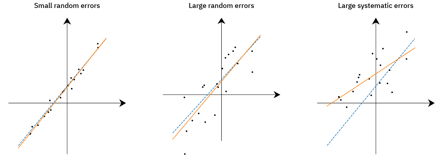
The dashed blue line is the reality we want to learn as accurately as possible. The orange line is a learned model based on the available training data (black dots). To the left, in case of small random (statistically unbiased) errors, the line can be learned well with little training data. In the middle, in case of larger still random (unbiased) errors, the line can still be learned well (the errors can be “generalized away”), but to achieve a good precision more training data is needed. To the right, in case of systematic (statistically biased) errors, the correct model cannot be learned no matter how much training data is available. Our experiment aimed to understand what type of errors are obtained in a real annotation process involving real human annotators - to what extent are they random and can be mitigated by more data (case in the middle panel), and to what extent are they systematic and lead the object detector systematically wrong (case in the rightmost panel)?
Experimental setup
We used a dataset from a client that has been annotated in Kognic production with our best quality with a well-defined annotation guideline, well-trained professional annotators and statistical quality checks. The dataset contained 3000 static images (frames) from a front-facing camera in various driving conditions, including highways and inner city driving. All vehicles and pedestrians were annotated with bounding boxes according to the annotation guideline. We refer to this dataset as Dataset A.
To obtain a second dataset with more errors, we also annotated the same set of frames with another workforce of professional annotators. We refer to this as Dataset B. The annotators of Dataset B were, however, neither trained for that type of two dimensional bounding box annotations nor that particular annotation guideline.
To understand the possible errors in dataset A and B, as well as how they impact a state-of-the-art object detector, we trained the object detector Detectron2 on both datasets. We refer to the one trained on dataset A as OD A, and the one trained on dataset B as OD B.
Comparing the performance of OD A & B
To evaluate the performance of OD A and OD B, we introduce a third dataset called dataset C. Dataset C is another dataset, with similar types of images, also annotated in production with our best quality. In terms of average precision, OD A scored 40.0 in predicting dataset C, whereas OD B scored a significantly lower 37.9.
The result indeed suggests that the quality of dataset B is inferior, but only looking at these two numbers does not tell us what type of errors there are in dataset B: are the errors just random and could be covered up by adding more training data, or are the errors so systematic that they are learned by the object detector and introduce an unrecoverable bias in its predictions?
To this end, we consider k-fold cross validation. By splitting dataset A and B into 5 folds each, and use 4 for training and 1 for validation, and repeating and averaging over all 5 such setups, we obtain an estimate on how well OD A and OD B would have performed in predicting another dataset annotated by the same annotation workforce. If the errors in dataset B were random (hard to predict), we would expect OD B to report a lower performance than OD A in this procedure. That was, however, not what we did see. OD A reported an average precision of 39.4, and OD B reported 39.3.
The very similar performance of both object detectors suggests that the differences between dataset A and B is merely a matter of systematic errors that are equally possible to learn and predict for the object detector, rather than different degrees of random errors that cannot be predicted. To better understand what these systematic errors are in practice, we take a closer look at the data and the annotations.
Characteristics from annotations that are inherited in the predictions
To more concretely see what the systematic differences are between dataset A and B, and to what extent they are replicated in the predictions by OD A and OD B, we will now walk through a set of statistics and visualizations of the annotations/predictions. The annotations are the training data (dataset A and B), whereas the predictions are the ones made by OD A and OD B for the input images in dataset C.
First we can simply count the number of objects that were found in each dataset/set of predictions.
In the annotations
- Dataset A contained 55 930 bounding boxes
- Dataset B contained 44 311 bounding boxes - 20% less
In the predictions
- OD A predicted 39 544 bounding boxes
- OD B predicted 34 028 bounding boxes - 14% less
At this very aggregated level, the behavior in the training data is clearly replicated (although slightly less emphasized) in the predictions; OD B was trained on data with fewer annotated objects, and thereby learned to detect fewer objects.
Since both dataset A and B contain the same images (just different annotations of them), we can compare the number of objects in them frame-by-frame, and similarly for the predictions by OD A and OD B for the new images of dataset C. The x-axis is the difference in number of objects between the same image (a number > 0 means dataset A/OD A found more objects than dataset B/OD B in the same image, and vice versa). If the annotations in dataset A and B had been identical, the figure would have had only a bar of height 3000 at 0.
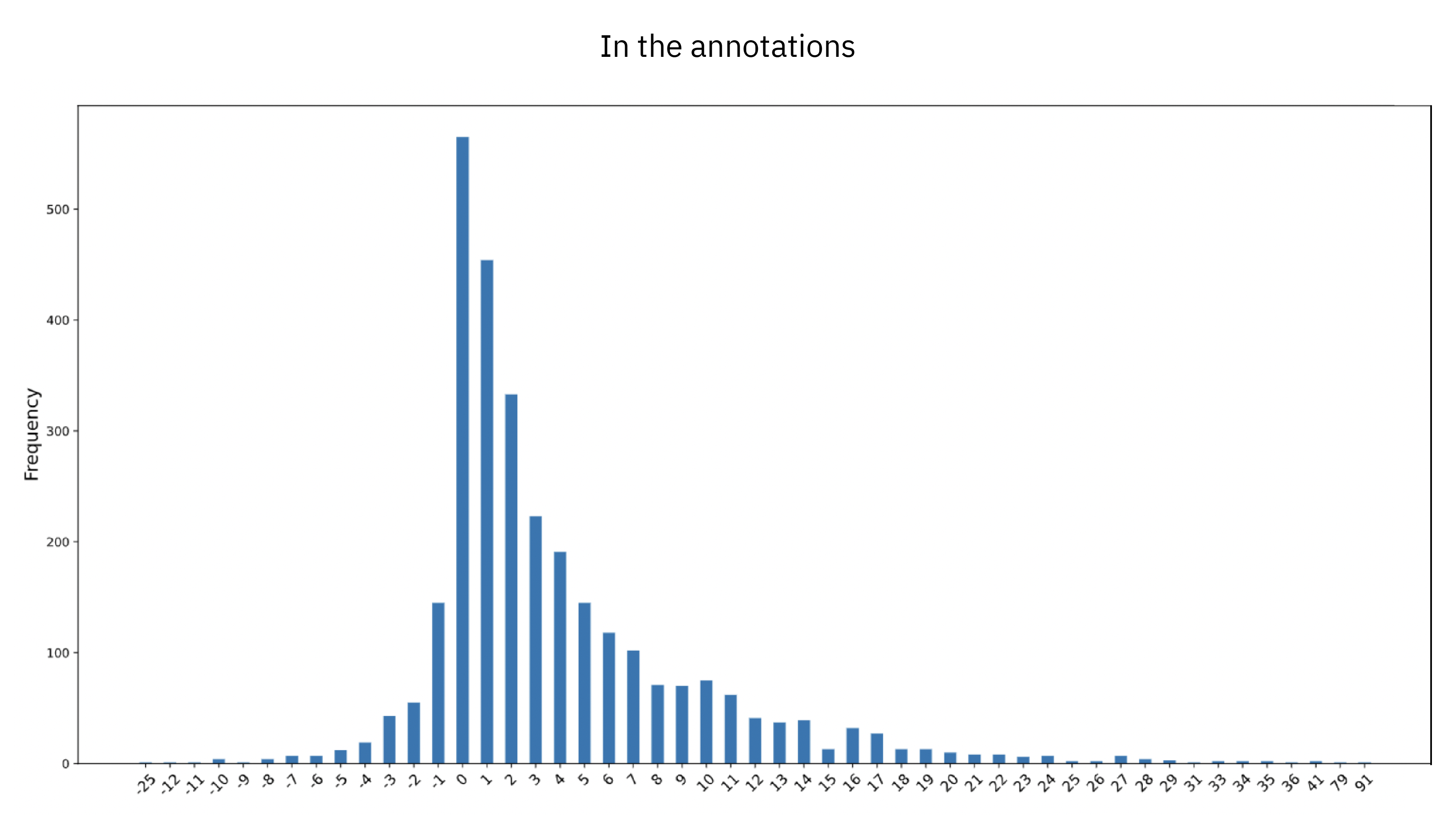
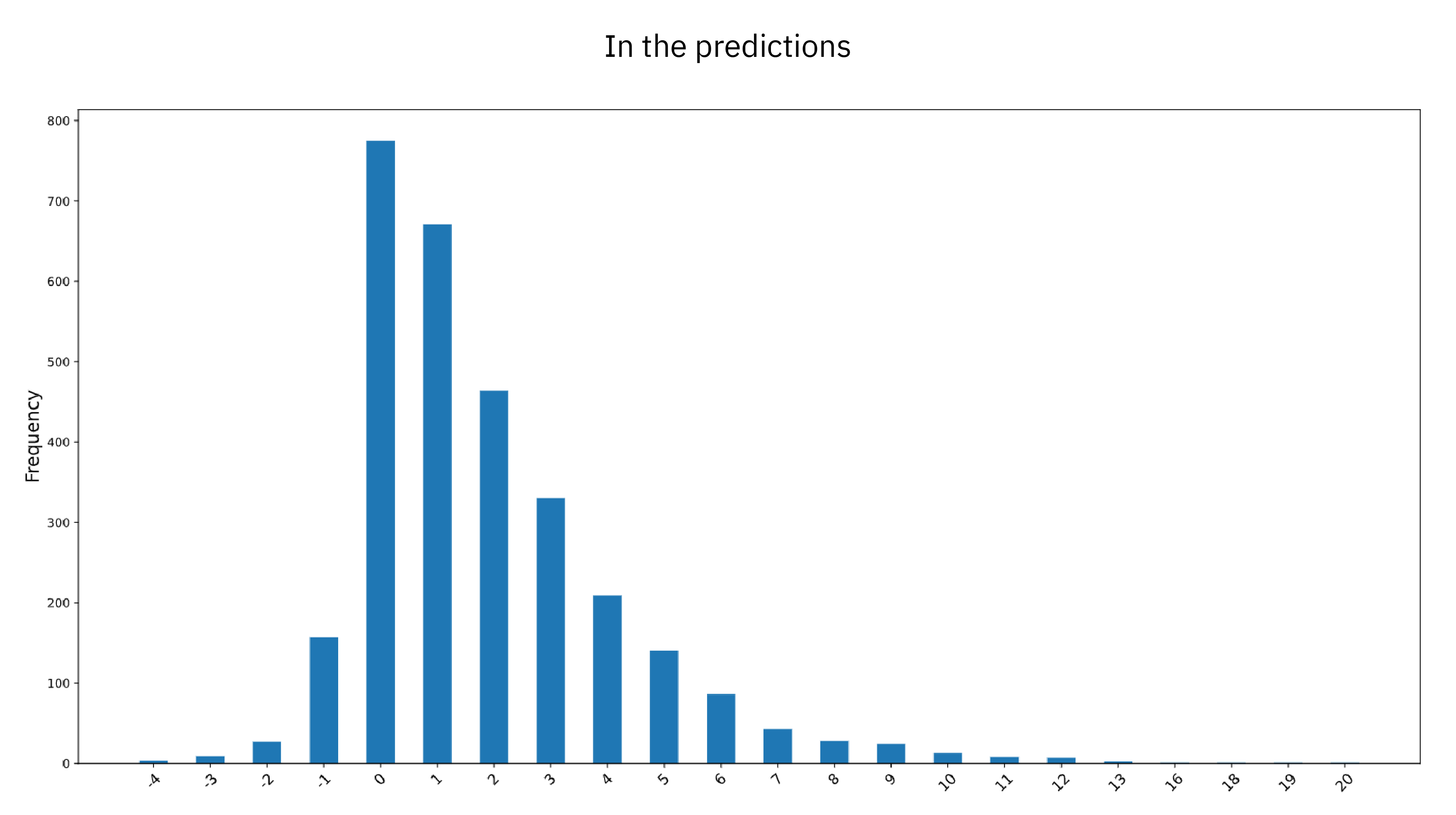
We see that in the annotations the most common case is an equal number of objects (0 difference), but also that in most frames in dataset A one or a few more objects are annotated than in dataset B. (The most extreme frame, with a difference in object count of 91 objects, is a scene with a parking lot next to the highway, that was carefully annotated in dataset A and completely ignored in dataset B.) Also from this perspective we see that the two object detectors have learned the characteristics of their respective training dataset, since the pattern is replicated also in the predictions (although a bit less pronounced; the largest differences are less extreme).
Moreover we can also see what sizes the annotated bounding boxes have. This figure shows two overlaid (not stacked) histograms with the distribution of bounding box sizes (measured as their areas in pixels) in dataset A and B, and the predictions of OD A and OD B, respectively.
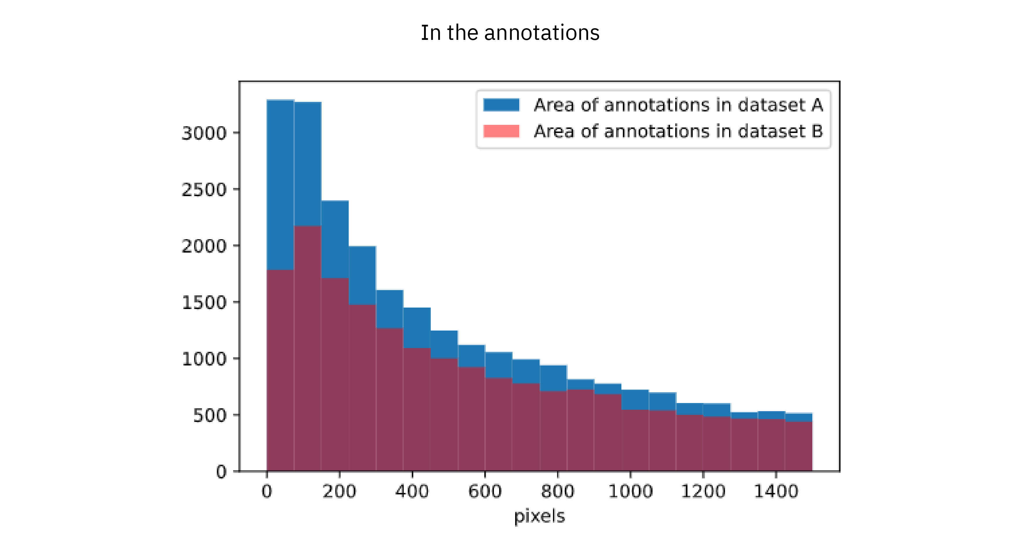
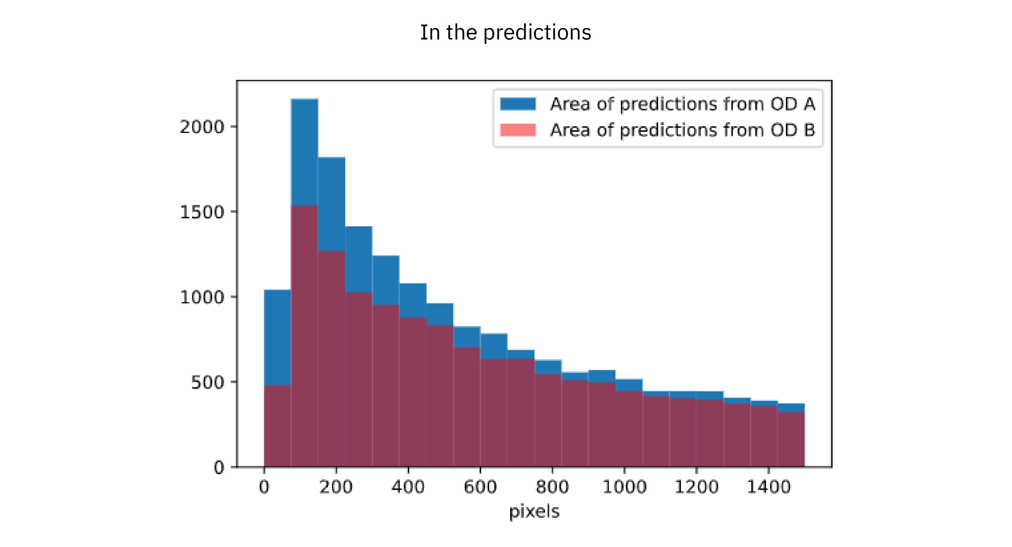
The main takeaway of the upper plot is that dataset A contains a larger proportion of smaller boxes than dataset B, suggesting that dataset B was annotated somewhat less carefully. This pattern is clearly replicated also in the predictions, where a larger proportion of smaller boxes are predicted by OD A than OD B. Again each object detector seems to have learned from how the training data was annotated.
We can dive even further into the analysis by comparing the individual bounding boxes from dataset A and B, and consider two boxes to match if the IoU (intersection over union) exceeds 0.7. In this way we get a picture of the difference between the individual boxes, which we can overlay on an example image. Although there were fewer boxes in dataset B than A, not all boxes in B were present in A. The annotators of dataset B also annotated certain objects that were not annotated in dataset A. We start with looking at these ones.
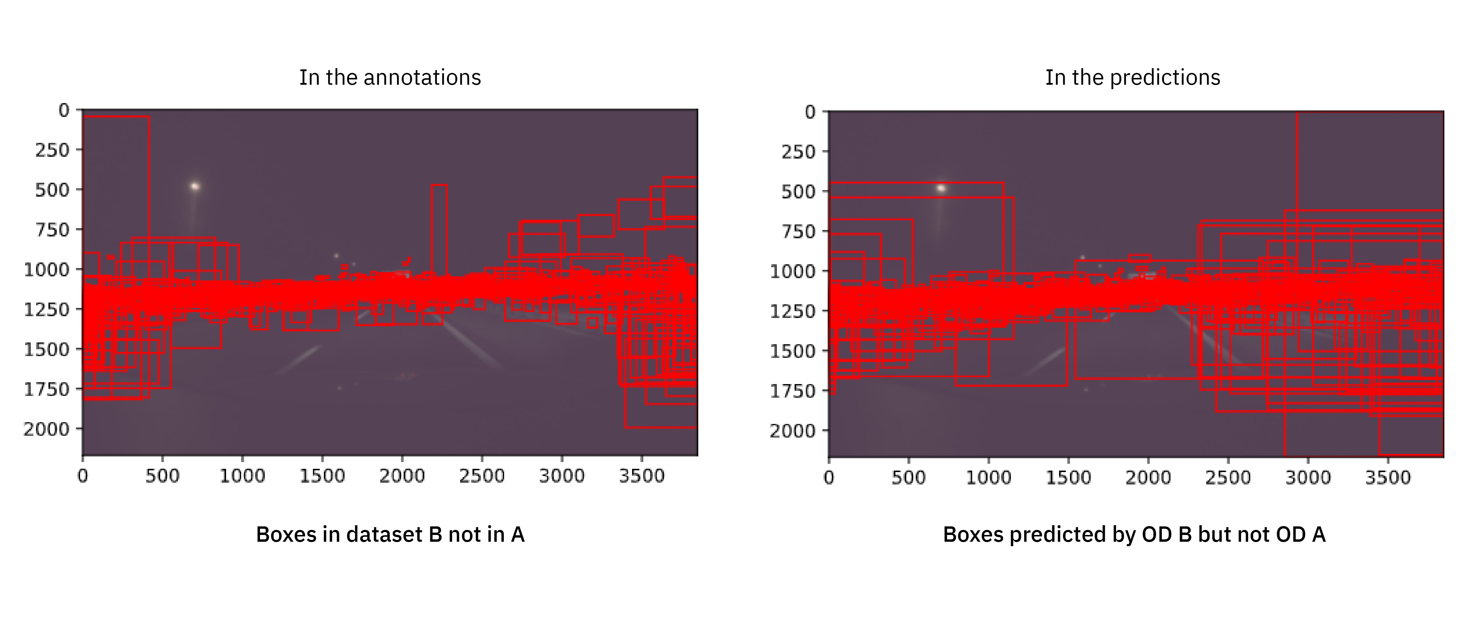
If we also compare these figures to the opposite ones, namely boxes in dataset A without a corresponding box in dataset B (and similarly for the predictions), we get the full picture.
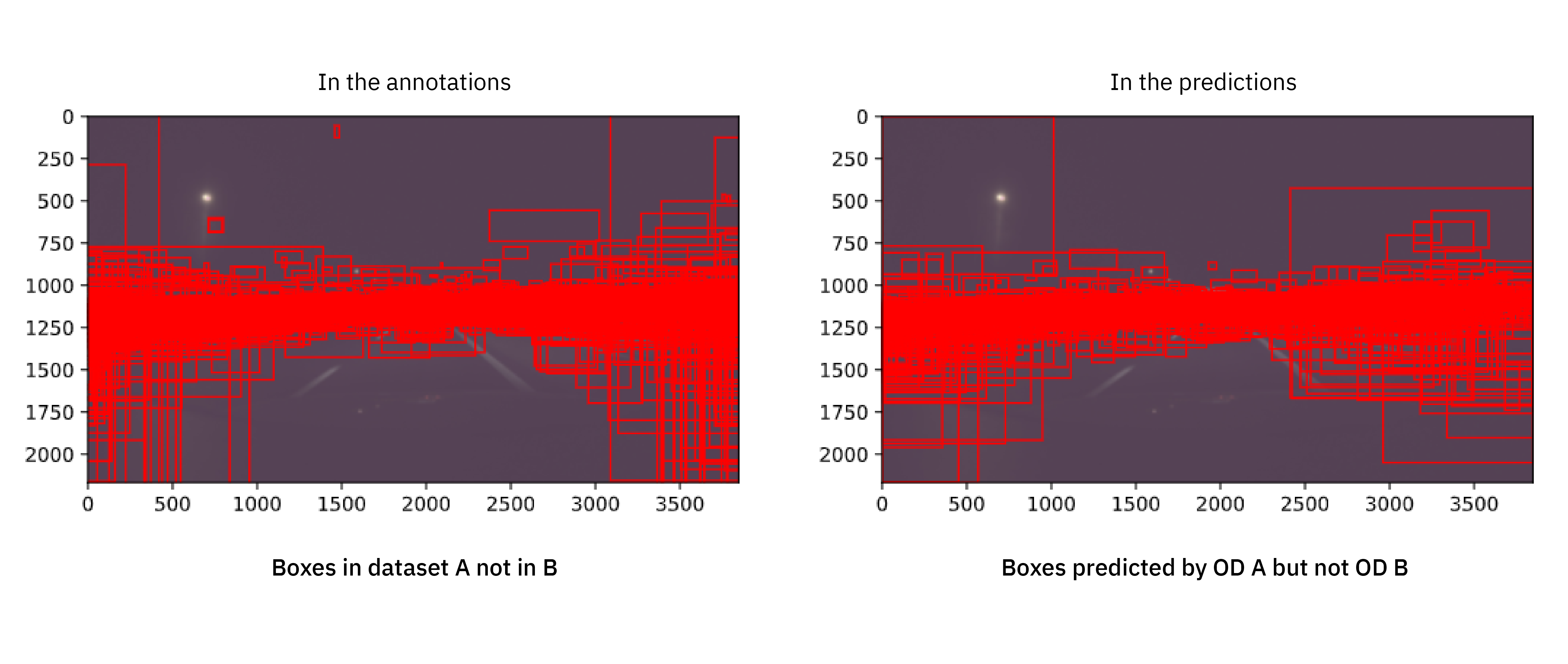
The first observation is that the vast majority of all differences in the annotations are concerning small distant objects. That is, the human annotators rarely disagree on what is right in front of the ego vehicle. While that is reassuring, it is also highlighting one of the ways in which annotation errors are systematic.
A second observation is that there is a clear visual resemblance between each of the annotation differences and corresponding prediction differences. The differences are not uniformly distributed neither over location nor size, but the “found by B not A” boxes are smaller and limited to a more narrow horizontal band than the “found by A not B” boxes, both in the training data and the predictions. Again, the characteristics of the errors in the annotations seem to have been learned by the object detector.
Finally we can also compare the differences in how the bounding boxes are drawn: even if the same object is annotated both in dataset A and B, or predicted by OD A and OD B, it can very well be indicated by bounding boxes of different sizes. We therefore compare, for each bounding box that matches (IoU > 0.7) between A and B, the difference between its borders (left, right, bottom, top) in the two datasets.
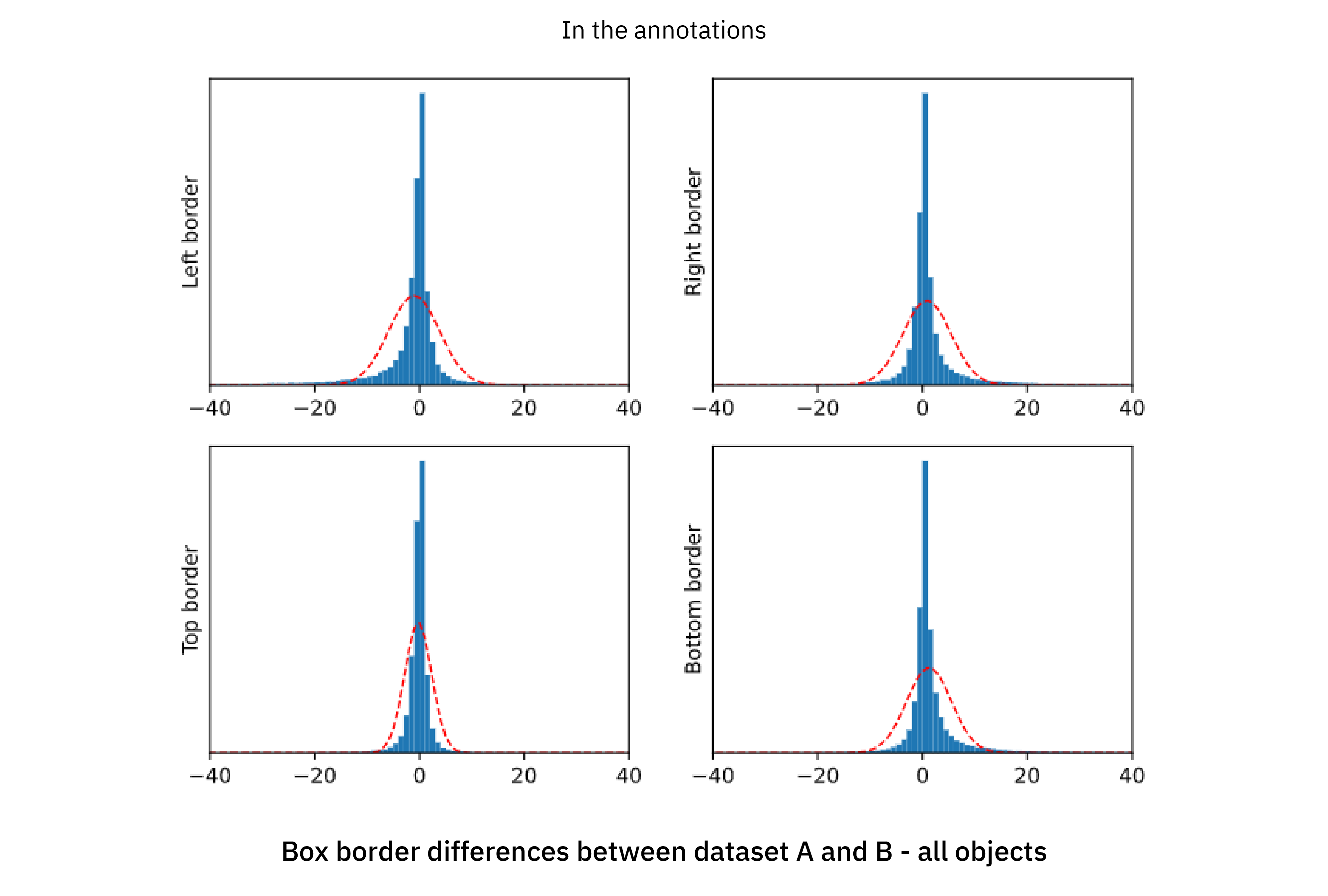
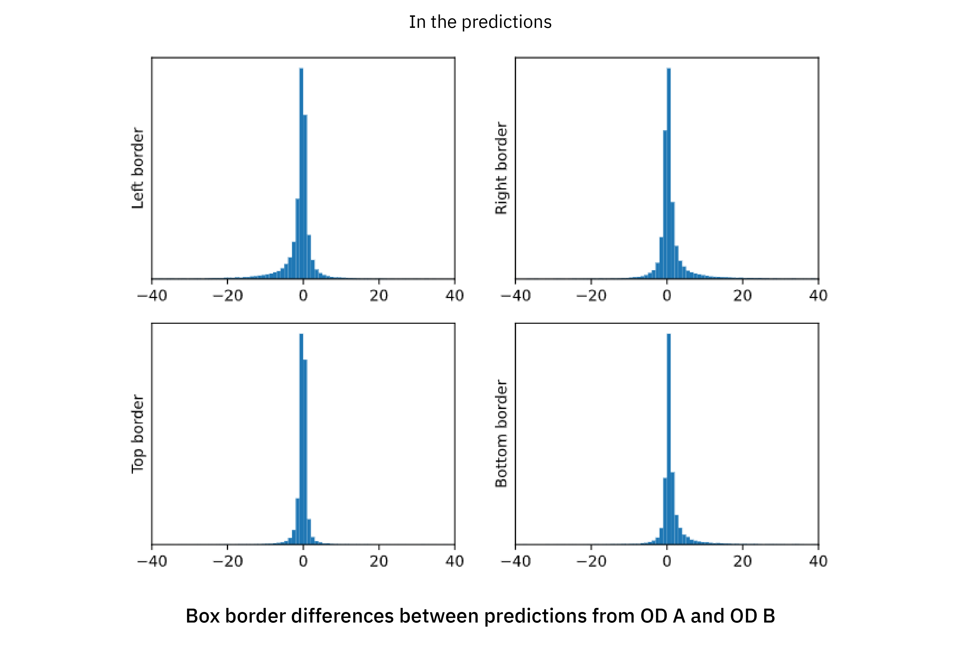
First looking at the upper part with annotations, the result is perhaps a bit surprising, in the sense that the distributions are asymmetric and almost exhibit a “spike and slab” pattern with a narrow peak (the “spike”) and a smeared-out part (the “slab”) which gives the distribution significant tails. To emphasize this point even more, a fitted Gaussian distribution is shown for reference. It is clear that the difference between the two annotations are not well described by a Gaussian distribution, and we can safely say that any realistic simulation of annotation errors in bounding box placement needs to use a more elaborate model.
By some further analysis, not included in this blogpost, we found that the “slab” was mostly attributed to objects that were not fully visible to the annotator. In other words, the tail of these plots represent the disagreement in the human process of extrapolating information, and the asymmetry is because of seemingly different strategies on how to handle that by the annotators of dataset A and B.
However, the most interesting observation is probably that the very same patterns are repeated in the predictions. Not only does the object detector adapt to what objects are annotated or not (the previous statistics/analysis points), it also learns the different strategies of how to draw the bounding boxes that are represented in dataset A and B respectively!
Conclusions
In this experiment we obtained two sets of annotations of the same images, dataset A and B. We did deliberately arrange the annotation of dataset B to obtain a lower quality. We could confirm that there were clear differences between dataset A and B, but whereas we could see that there were systematic differences in the annotations, we were unable to claim a different rate of random errors between the two datasets: According to the k-fold cross validation analysis, the annotations of both datasets were equally possible to predict by an object detector. There might indeed be a certain amount of random errors present in both dataset A and B, but we can not see a larger presence of them in dataset B despite its lower quality.
Our first conclusion is therefore that, contrary to popular belief, the difference between a carefully and a less carefully annotated dataset is not well described by randomly injected errors; this experiment suggests that most low-quality annotation artefacts are more systematic in nature. We find no support for that studies of the type “remove 10% of all boxes randomly and see what effect it has when training an object detector” gives any realistic insights when it comes to deciding on what annotation quality to use.
Our second conclusion is that the systematic annotation errors were learned by the object detector and present also in its predictions, although sometimes slightly less pronounced. There was no indication that the object detector would have been able to “generalize away” the errors in dataset B, had it only been given more low-quality training data.
We would therefore like to caution on using low-quality training data for training safety-critical perception systems: we have seen that consciously lowering the annotation quality introduced little random errors, but a substantial amount of systematic errors. Chances are that any low-quality data contains certain subtle hard-to-find systematic errors that are learned as a policy by a machine learning model and from there directly inherited into its predictions. There is no reason to believe such errors can be covered up by adding more low-quality data possibly containing the same systematic error.
Share this
Written by


